深度学习 卷积 笔记
本文最后更新于:2023年6月15日 下午
一些理解
用神经网络去学习构建卷积核
卷积层将输入和核矩阵进行交叉相关,加上偏移之后得到输出。
核矩阵和偏移是可学习的参数
核矩阵的大小是超参数(在训练前就已经定义好)
比较好的思想:高、宽减半,通道数翻一倍
二维交叉与二维卷积
没有本质的区别,
\(y_{i,j}=\sum_{a=1}^{h}\sum_{b=1}^{w}w_{a,b}x_{i+a,j+b}\)
索引前多了负号,因为w是学习的值,所以没有本质区别
\(y_{i,j}=\sum_{a=1}^{h}\sum_{b=1}^{w}w_{-a,-b}x_{i+a,j+b}\)
不同的维度
一维
\(y_i=\sum_{a=1}^hw_ax_{i+a}\)
处理文本、语言、时间序列
三维
\(y_{i,j,k}=\sum_{a=1}^h\sum_{b=1}^w\sum_{c=1}^d\)
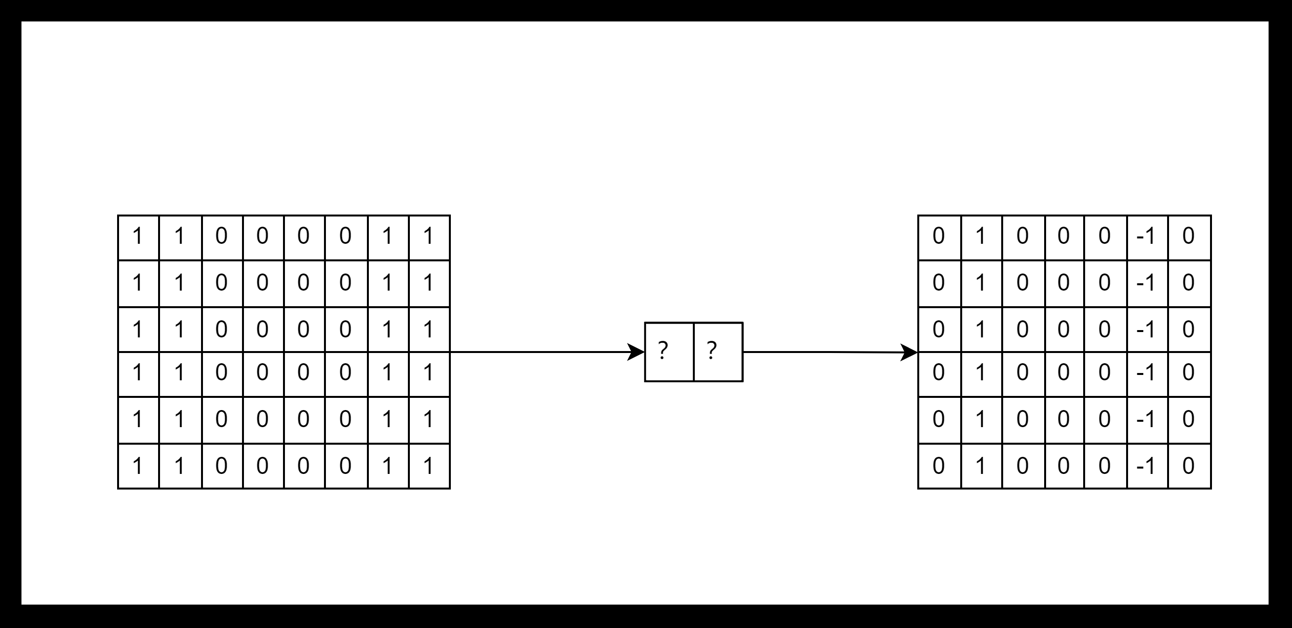
实现二维卷积层
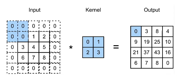
互相关运算
1 | |
1 | |
例子
1 | |
填充和步幅
原因
每次使用卷积核都能减小输出的大小
input:32x32kernel_size:5x5- 根据
kernel_size每卷积一次,减少4x4 - 第一次卷积
32x32:arrow_right:28x28 - ...
- 第七次卷积结果
4x4
- 根据
- 总结:每卷积一次,形状从\(n_h \times
n_w\)减小到\((n_w-k_h+1)\times(n_w-k_w+1)\)
- 其中
k_h为卷积核的高,k_w为卷积核的宽
- 其中
填充
在输入数据的四周进行数据填充。
- 在上下左右分别添加0
- 输出形状为\((n_h-k_h+p_h+1) \times(n_w-k_w+p_w+1)\)
- 通常取 \(p_h=k_h-1\),\(p_w=k_w-1\)
k为奇数,在上下两侧填充\(p_h/2\)k为偶数,在上侧填充\([p_h/2]\),在下侧填充\([p_h/2]\)
步幅
控制卷积核移动的幅度,可以每次不止移动一格。
可以使得在输入较大、卷积核较小的情况下,快速达到较小的输出,减少中间的卷积层数。
- 给定高度\(s_h\)和宽度\(s_w\)的步幅,输出形状为:\([(n_h-k_h+p_h+s_h)/s_h]\times[(n_w-k_w+p_w+s_w)/s_w]\)
- 如果 \(p_h=k_h-1\),\(p_w=k_w-1\),输出形状为:\([(n_h+s_h-1)/s_h]\times[(n_w+s_w-1)/s_w]\)
- 如果输入高度和宽度可以被步幅整除,输出形状为:\((n_h/s_h)\times(n_w/s_w)\)
总结
- 填充和步幅都是卷积层的超参数,声明网络的时候加上就行
- 填充在输入周围添加额外的行/列,来控制输出形状的减少量,常设为
p = k-1核-1 - 步幅是每次滑动核窗口时的行/列的步长,可以成倍地减少输出形状
例子
1 | |
输入和输出通道
每个通道有自己的卷积核
\(c_i\):输入通道
channel_input
\(c_o\):输出通道channel_output
单输入通道
每个通道和自己的卷积核进行计算
- 输入
X:\(c_i\times n_h\times n_w\) - 核
W:\(c_i\times k_h\times k_w\) - 输出
Y:\(m_h\times m_w\)
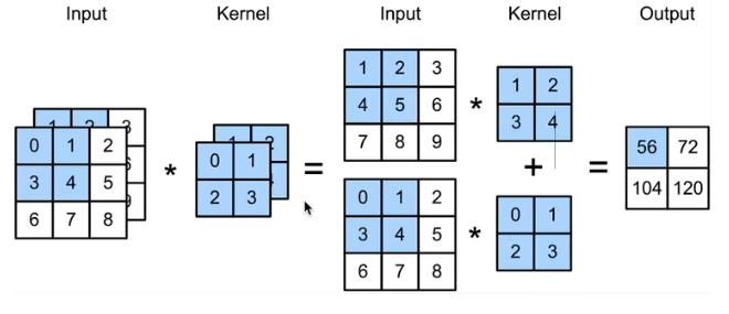
多输入通道
多个卷积核、每个核生成一个通道
每个通道可有用于识别不同的特定模式
- 输入
X:\(c_i\times n_h\times n_w\) - 核
W:\(c_o\times c_i\times k_h\times k_w\) - 输出
Y:\(c_o\times m_h\times m_w\)
1 | |
1 | |
1x1卷积层
参考:一文读懂卷积神经网络中的1x1卷积核 (qq.com)
不识别空间模式(没有周边像元参与),只是对多个通道同一位置的像元进行融合
\(k_h=k_w=1\)
相当于输入形状为\(n_hn_w\times c_i\),权重为\(c_o\times c_i\)的全连接层
- \(z=W\cdot x^T+b\)
- \(W: \space c_o \times c_i\)
- \(x:\space n_hn_w \times c_i\)
- 对应位置按权重(
Kernel)相加
1 | |
总结
- 输出通道数是卷积层的超参数
- 每个输入通道有独立的二维卷积核,所有通道结果相加得到一个输出通道结果
- 每个输出通道有独立的三维卷积核
[3,2,2,2]输出通道为3,输入通道为2,卷积核高2,卷积核宽2- 有三个卷积核,每个卷积核有两层(是二维),卷积核大小为2x2
池化
二维最大池化
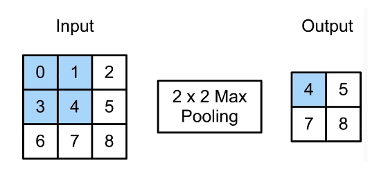
返回滑动窗口中的最大值
- 有填充和步幅
- 没有可学习的参数,只有取最大的操作子
- 每个输入通道应用池化层获得相应的输出通道
- 输入通道数=输出通道数
二维平均池化
- 和最大池化一样,操作子变为取平均
1 | |
1 | |
总结
- 池化层返回窗口中的最大或者平均值,取决于操作子
- 池化层能缓解卷积层对位置的敏感性
- 同样有窗口大小、填充和步幅作为超参数
卷积层、全连接层参数个数计算
- 卷积层参数量:卷积核元素的大小
- 计算公式:参数量=(filter size * 前一层特征图的通道数 )* 当前层filter数量
- 全连接层参数量:
- 计算公式:见参考
批量归一化
问题
底部:靠近数据
顶部:靠近损失
训练过程中,方差和均值的分布在不同层之间发生变化
在持续的训练过程中,上面的收敛比较快,下面变化比较慢。
但是每次底部变化,底层的信息变了,顶部需要进行重新训练。
这个问题会导致收敛比较慢。
原因
- 损失在网络计算的最后(上部),网络后面的层的训练比较快
- 数据在网络的最底部
- 底层训练很慢
- 底层变化,整个网络的数据都发生变化
- 最后的那些层需要学习很多次
- 导致收敛变慢
解决方法
把不同层之间的均值和方差的分布固定住。
固定小批量里的均值和方差
\(\begin{split}\begin{aligned} \hat{\boldsymbol{\mu}}_\mathcal{B} &= \frac{1}{|\mathcal{B}|} \sum_{\mathbf{x} \in \mathcal{B}} \mathbf{x},\\ \hat{\boldsymbol{\sigma}}_\mathcal{B}^2 &= \frac{1}{|\mathcal{B}|} \sum_{\mathbf{x} \in \mathcal{B}} (\mathbf{x} - \hat{\boldsymbol{\mu}}_{\mathcal{B}})^2 + \epsilon.\end{aligned}\end{split}\)
\(\mathrm{BN}(\mathbf{x}) = \boldsymbol{\gamma} \odot \frac{\mathbf{x} - \hat{\boldsymbol{\mu}}_\mathcal{B}}{\hat{\boldsymbol{\sigma}}_\mathcal{B}} + \boldsymbol{\beta}.\)
\(\gamma \quad \beta\) 可学习的参数,当变为标准正态分布可能不太合适的话,可以用数据重新学习一个合适的方差和均值对数据进行优化。
批量归一化层
- 可学习的参数为\(\gamma\quad\beta\)
- 作用在
- 全连接层和卷积层输入上
- 全连接层和卷积层输出上,激活函数之前
- 对输出数据减去均值除以方差,加上可以学习的\(\gamma\quad\beta\),在加上激活函数
- 对于全连接层,作用在特征维
- 全连接层输入是二维的
- 行是样本,列是特征。
- 作用在特征维度是对特征求均值和方差(列)
- 对于卷积层,作用在通道维
- 二维拓展到三维
Batch size x Channels x Height x Width- 样本数量:
Batch size x Height x Width个像素 - 每个像素:
Channels个通道(特征)
- 样本数量:
- 对每个像素的通道计算均值和方差
代码
1 | |
1 | |
1 | |
1 | |
总结
- 批量归一化固定小批量中的均值和方差,然后学习出合适的偏移和缩放
- 可以加速收敛速度,但是一般不改变模型精度
- 可以允许用更大的学习率进行训练
LeNet 经典卷积神经网络
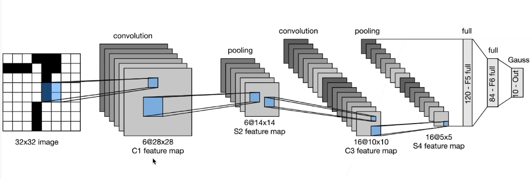
1 | |
AlexNet 卷积神经网络
特点
更大更深的LeNet

主要改进
- 丢弃法
ReLUMaxPooling
代码
1 | |
1 | |
VGG 使用块的网络
特点
更深更窄
- 堆更多的
3 x 3的卷积核
VGG块
n层,m通道的卷积层- 最后加个
2 x 2的最大池化层
VGG架构
AlexNet整个卷积层的架构替换为n个VGG块,VGG-16,VGG-19- 块可重复使用,不同的卷积块个数和超参数可以得到不同复杂程度的变种
代码
1 | |
1 | |
1 | |
1 | |
1 | |
NiN 神经网络
原因
- 卷积层参数个数: \(c_i \times c_o \times k^2\)
- 卷积层后第一个全连接层参数个数:
- 相当于用
output_channels个\(1\times1\)的卷积核进行卷积计算 - \(c_i \times c_o \times k^2\)
- 相当于用
块架构
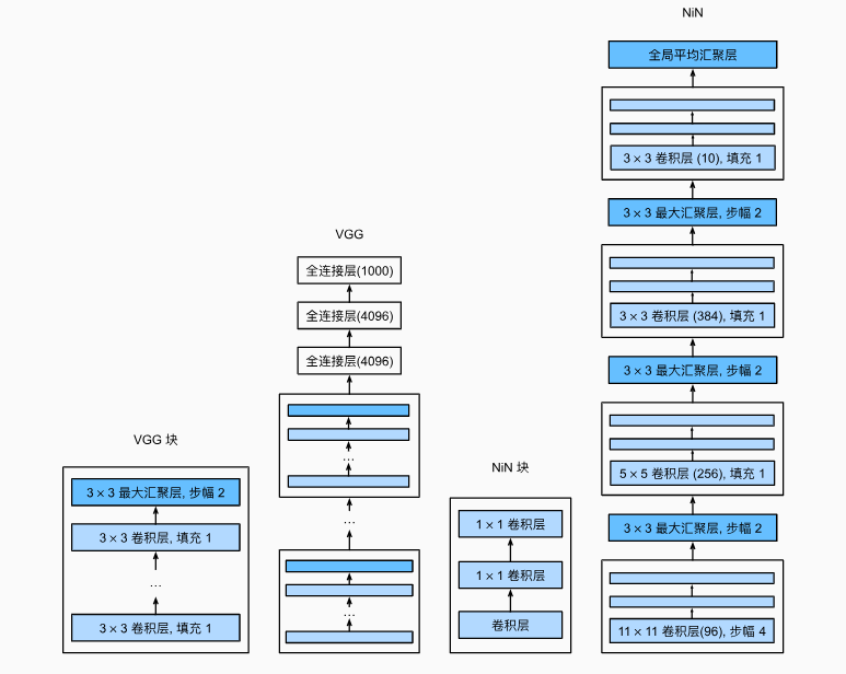
- 一个卷积层后跟两个全连接层
- 步幅为1,无填充,输出形状跟卷积层输出一样
- 起到全连接层的作用
特点
- 无全连接层
- 交替使用NiN块和步幅为2的最大池化层
- 逐步减少高宽(减半)和增大通道数(加倍)
- 最后使用全局平均池化层得到输出
- 输入通道数是类别数
- 池化层的高宽=原始输入的高宽
代码
1 | |
1 | |
1 | |
1 | |
GoogLeNet 网络
特点
引入了
Inception块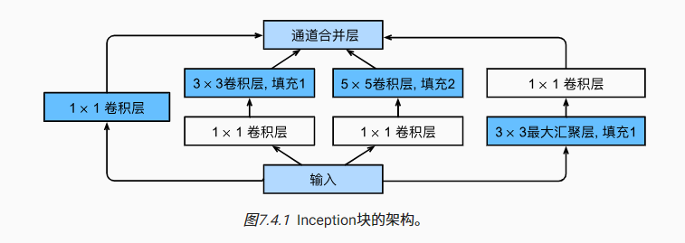
Inception块由四条并行路径组成。 前三条路径使用窗口大小为1×1、3×3和5×5的卷积层,从不同空间大小中提取信息。 中间的两条路径在输入上执行1×1卷积,以减少通道数,从而降低模型的复杂性。 第四条路径使用3×3最大汇聚层,然后使用1×1卷积层来改变通道数。 这四条路径都使用合适的填充来使输入与输出的高和宽一致,最后我们将每条线路的输出在通道维度上连结,并构成Inception块的输出。在Inception块中,通常调整的超参数是每层输出通道数。基于
Inception块,构建了网络
代码
1 | |
1 | |
1 | |
1 | |
ResNet 残差网络
特点
保证新加入的层的使得效果至少不会变差
残差块
- 串联一个层改变函数类,扩大函数类
- 残差块加入快速通道得到\(f(x) = x + g(x)\)的结构

原来的向后传播,或者加入一个1x1卷积层来变换通道数量使得能够继续向后
- 即使中间的块什么都没有学到,之前的层的结果还是能够继续向后传播
- 类似VGG和GoogLeNet的总体架构,但是替换成了ResNet块
种类
- 高宽减半
ResNet块(步幅为2) - 后接多个高宽不变
ResNet块
代码
1 | |
1 | |
1 | |
总结
- 残差块使得很深的网络更加容易训练
- 后面的网络或多或少都有残差块的思想
- 下面小的先训练好,再训练深的,因为有跳转层