深度学习 计算机视觉 笔记
本文最后更新于:2023年7月5日 凌晨
边缘框
实现
1 | |
执行
1 | |
锚框
原理
锚框与边框
- 边框 bounding box bbx 真实值
- 锚框:预测框
特点
- 是一类目标检测算法
- 提出多个被称为锚框的区域
- 预测每个锚框内是否含有关注的物体
- 如果是,预测从这个锚框到真实边缘框的偏移
IoU 交并比
- 衡量两个框之间的相似度
- 约定两个集合
A,B- \[J(A,B)=\frac{|\mathbf A\cap \mathbf B|}{|\mathbf A\cup \mathbf B|}\]
- 0表示有无重叠,1表示有重叠
赋予锚框标号
- 每个锚框是一个训练样本
- 每个锚框,要么标注成背景,要么关联上一个真实边缘框
- 缺点
- 可能会生成大量的锚框,导致大量的负类样本
使用非极大值(NMS)抑制输出
- 每个锚框预测一个边缘框
- NMS可以合并相似的预测
- 选中是非背景类的最大预测值
- 去掉所有其它和它IoU值大于\(\theta\)的预测
- 重复上述过程,要么预测被选中,要么被去掉
锚框生成方式
- 以每一个像素为中心
- 生成不同高度、宽度的锚框
- 锚框的宽度和高度分别为\(ws\sqrt{r}\)和\(hs/\sqrt{r}\)
s和r的取值,不是阶乘组合,而是只考虑包含s1或者r1的组合n+m-1size+ratio-1- \((s_1, r_1), (s_1, r_2), \ldots, (s_1, r_m), (s_2, r_1), (s_3, r_1), \ldots, (s_n, r_1).\)
总结
- 一类目标检测算法基于锚框来预测
- 首先生成大量锚框,并赋予标号,每个锚框作为一个样本进行训练
- 在预测时,使用NMS来去掉冗余的预测
代码实现
引入库并设置精度
1 | |
锚框的宽度和高度分别为\(ws\sqrt{r}\)和\(hs/\sqrt{r}\)
w照片宽度,h照片高度s:scale,锚框占照片大小的百分比r:ratio ,锚框的高宽比
物体检测算法
R-CNN
Region-CNN

特点
- 使用启发式搜索算法
selective search来选择锚框 - 使用预训练模型
pretraining-mode对每个锚框抽取特征 - 训练一个SVM来对类别分类
- 训练一个线性回归模型来预测边缘框偏移
一个图片变为一千张小图片 ,计算量很大
RoI Pooling 兴趣区域池化层
- 给定一个锚框,均匀分割为
nxm块,输出每块里的最大值。- 每个锚框的大小不同,但是作为分类依据的时候需要变为相同的大小,作为
batch
- 每个锚框的大小不同,但是作为分类依据的时候需要变为相同的大小,作为
- 不管锚框多大,总是输出
nm个值
具体流程
- 对输入图像使用选择性搜索来选取多个高质量的提议区域(
proposal region) (Uijlings et al., 2013)。这些提议区域通常是在多个尺度下选取的,并具有不同的形状和大小。每个提议区域都将被标注类别和真实边界框; - 选择一个预训练的卷积神经网络,并将其在输出层之前截断。将每个提议区域变形为网络需要的输入尺寸(
RoI Pooling),并通过前向传播输出抽取的提议区域特征; - 将每个提议区域的特征连同其标注的类别作为一个样本。训练多个支持向量机对目标分类,其中每个支持向量机用来判断样本是否属于某一个类别;
- 将每个提议区域的特征连同其标注的边界框作为一个样本,训练线性回归模型来预测真实边界框。
Fast RCNN
特点
- 使用CNN对图片进行特征抽取
- 使用ROI池化层对每个锚框生成固定长度特征
SSD
结构

基础网络块
2 x 3 x 256 x 256 --> 2 x 64 x 32 x 32 作用:抽特征,获取feature map(Y) 2 x 64 x 32 x 32
锚框生成
multibox_prior(data,size,ratio) 作用:根据data的高、宽以及锚框的size ratio生成锚框 32 x 32 x (3+2-1)
类别预测
cls_predictor(Y) 作用:根据feature map预测每个像素的锚框可能的类别 32 x 32 x (3+2-1) x (1+1)
边界预测
box_predictor(Y) 作用:根据feature map 预测每个锚框的位置 32 x 32 x (3+2-1) x 4
理解
特征图 2 x 64 x 32 x 32
用 cls_predictor Conv2d(64,8,kernel=3,padding=1) 从特征图中抽出8类作为新的特征
- 输出通道为8,8个滤波器
- 每个滤波器 卷积核 3 x 3 x 64
- 专门抽类别特征的,卷积核里的参数慢慢训练为可以做类别分类的
用 box_predictor Conv2d(64,16,kernel=3,padding=1) 从特征图中抽出16个偏置(4x4)作为新的特征
- 输出通道为16,16个滤波器
- 每个滤波器 卷积核 3 x 3 x 64
- 专门抽偏置特征的,卷积核里的参数慢慢训练为可以获取偏置的
无论输入图像的通道是多少,每经过一个滤波器都将生成一个通道为1的特征图。
一个卷积层之内可定义多个滤波器,当前卷积层上的各个滤波器会对上一层输入的每个feature map(特征图)分别执行卷积操作,即每个滤波器都会对应生成一个新的特征图feature map(不同的滤波器所提取的特征不同)。
故而在下一层需要多少个特征图,本层就需要定义多少个滤波器,即滤波器的个数与传出的特征图的张数一致。
代码
1 | |
1 | |
1 | |
1 | |
1 | |
1 | |
1 | |
1 | |
1 | |
1 | |
1 | |
1 | |
1 | |
1 | |
1 | |
1 | |
语义分割
转置卷积
特点
- 普通卷积算子不会增大输入的高、宽,通常要么不变,要么减半
- 转置卷积可以用来增大输入的高宽
原因
- 常用的卷积算子算到最后像素级别的数据被压缩到很小的范围
- 但是语义分割需要输出像素级别精度的类别,所以需要数据扩充

概念
- 转置卷积是一种计算方式
- 卷积一般做下采样,转置卷积一般做上采样
- 意义在于
- 如果你使用某种卷积使得输入\((h,w)\)变为\((h',w')\)
- 那么你可以使用同样超参数的转置卷积,使得输入\((h',w')\)变为\((h,w)\)
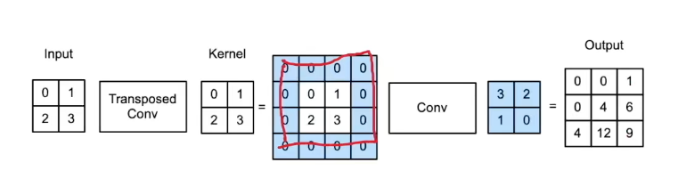
- 填充为0 步幅为1
- 计算方式1
- 将输入填充
k-1 - 将核矩阵上下、左右翻转
- 做正常卷积(填充0,步幅1)
- 将输入填充
- 计算方式2
- 按转置卷积的方式计算
- 计算方式1
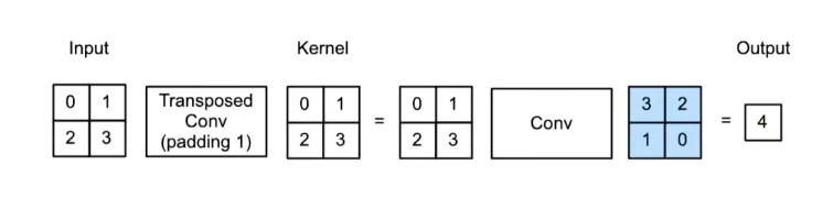
- 填充为p 步幅为1
- 计算方式1
- 将输入填充
k-p-1 - 将核矩阵上下、左右翻转
- 然后做正常卷积(填充0,步幅1)
- 将输入填充
- 计算方式2
- 按转置卷积的方式计算
- 在转置卷积的结果上去掉padding=1(外围一层)
- 计算方式1
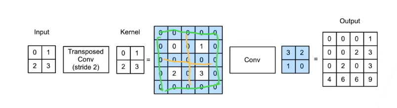
- 填充为p 步幅为s
- 计算方法1
- 在行和列之间插入
s-1行或列 - 将输入填充
k-p-1 - 将核矩阵上下、左右翻转
- 然后做正常卷积(填充0,步幅1)
- 在行和列之间插入
- 计算方法2
- 按转置卷积的方式计算
- 计算方法1
- 形状换算
- 输入高(宽)为
n,核k,填充p,步幅s - 转置卷积:
n'=sn+k-2p-s- 卷积:
n'=[(n-k-2p+s)]/s
- 卷积:
- 如果让高、宽成倍增加
k=2p+s
- 输入高(宽)为
总结
- 转置卷积是一种变化了输入和核的卷积,用来达到上采样的目的
- 不等同于数学上的反卷积操作 ##### 案例
1 | |
1 | |
填充
与常规卷积不同,在转置卷积中,填充被应用于的输出(常规卷积将填充应用于输入)。
例如,当将高和宽两侧的填充数指定为1时,转置卷积的输出中将删除第一和最后的行与列。
1
2
3
4
5
6
7
8
9
10
# 填补Padding
# Padding = 1
# 原过程:在“输出”的基础上 上下填补计算普通卷积得到“输入”
# 转置卷积过程:输入计算转置卷积再去掉上下填补的部分
# padding=1 把不含padding转置卷积的结果除掉padding
tconv = nn.ConvTranspose2d(1,1,kernel_size=2,padding=1,bias=False)
tconv.weigth.data = K
tconv(X)
1 | |
1 | |
全卷积网络(FCN)
定义
全卷积网络将中间层特征图的高宽变换回输入图像的尺寸。 最后的通道维输出该位置对应像素的类别预测。
构造
全卷积网络先使用卷积神经网络抽取图像特征,然后通过卷积层将通道数变换为类别个数,最后在通过转置卷积层将特征图的高和宽变换为输入图像的尺寸。 因此,模型输出与输入图像的高和宽相同,且最终输出通道包含了该空间位置像素的类别预测。
特点
双线性插值常用于初始化转置卷积层
代码
1 | |
1 | |
1 | |
1 | |
1 | |
1 | |
1 | |
1 | |
样式迁移学习

思想
- 一套网络复制三次,三个卷积层
- 合成图像的像素值是最后的训练目标
- 损失计算
- 合成图像与样式图像计算样式损失
- 合成图像与内容图像计算内容损失
- 最后损失用权重汇总为总变差损失作为优化目标
代码
1 | |
1 | |
1 | |
1 | |
1 | |
1 | |
1 | |
1 | |
1 | |
1 | |
1 | |
1 | |